From 52% to 58%: A Transformer Static Evaluator That Plays Like a 2-Ply Sim
In June 2025 I wrote about a convolutional neural network that beat HastyBot, our fast static evaluator, 51.7% of the time. I called it “just the beginning” and finished with a list of ideas: more heads, better data, maybe an NNUE, maybe plugging the net into BestBot.
This post is the sequel. The new network, macondo-tf, beats HastyBot 57.65% of the time, measured over 100,000 game pairs. That’s a big jump in Scrabble terms. More surprising to me: it’s as strong as a 2-ply Monte Carlo simulation of 100 candidate plays, while spending about 6 milliseconds per move instead of about 10 CPU-seconds.
Like last time, this is partly a story and partly documentation for future me. Every number here comes from our experiment log (pytorch/experiments.md and pytorch/RUNS.md in the Macondo repo). And like last time, a lot of what we tried didn’t work. I’ll show those too, because the dead ends taught us more than the wins.
Where we left off: the CNN plateau
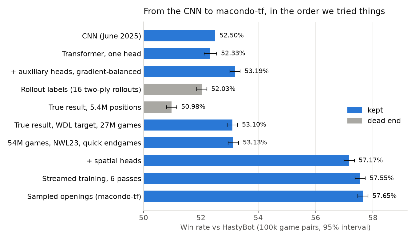
After that first post the CNN kept improving a little: a TensorRT fp16 build, more games, a bigger network. It topped out at about 52.5% against HastyBot. Then it stopped moving. I swept the width of the network from 64 to 128 channels and every version landed within 0.15% of the others:
128-ch: 52.45%
 96-ch: 52.55%
 80-ch: 52.50%
 64-ch: 52.39%
When four very different network sizes give the same answer, the network isn’t the bottleneck. Something else is.
How we measure now: game pairs
One methodology change first, because every number below depends on it. Scrabble is noisy. In the first post I reported raw win rates over a few hundred thousand games, with error bars that were sometimes bigger than the effects I was chasing.
Now every match is played in pairs. Each random seed is played twice, with the two bots swapping seats, so both bots see the same tile draws. Lucky draws mostly cancel out. A match is 100,000 pairs (200,000 games), and the paired 95% interval comes out to about ±0.18 points. That’s tight enough to see a 0.3-point improvement, and to say with some confidence when something did nothing.
The bot is the same simple one as before. FastMlBot generates HastyBot’s top 50 plays by static equity, asks the network to score each of them, and plays the best one.
The headline number doesn’t rest on my setup alone: John O’Laughlin, one of the authors of MAGPIE, confirmed macondo-tf’s win rate independently.
Step 1: a transformer (52.33%)
Some quick background first. The transformer is the architecture behind today’s large language models, introduced in the landmark 2017 paper “Attention Is All You Need”. Its input is a sequence of tokens, and its core operation is attention: in each layer, every token looks at every other token and decides which ones matter to it. In a language model the tokens are pieces of words, and attention is how a word near the end of a sentence finds the noun it refers to near the start. CNNs work differently: each layer only mixes a small neighbourhood, and information crawls across the board a few squares per layer.
There’s something fitting about the switch. An architecture invented to read words now judges a game about words, without knowing a single one: our net never sees the dictionary, only letters on squares and which letters each empty square will take.
Two people suggested switching from a CNN to a transformer: David Shin (Scribblez), who had his own value net beating HastyBot by more than 54%, and Morris Greenberg. The argument: attention handles “global” state much better than a conv stack. The CNN only sees the rack and bag after a global average pool flattens the board. A transformer lets every square look at the rack and the unseen tiles directly.
The transformer takes exactly the same inputs as the CNN: 85 board planes and 72 scalars. It turns them into tokens inside the model:
- 1 summary (CLS) token
- 225 square tokens, one per board square
- 27 tile-type tokens (how many of each letter we hold, and the chance of drawing it)
- 1 game-state token
That’s 254 tokens through 8 transformer layers with model width 192 and 6 attention heads, about 3.7M parameters (the CNN had 1.7M).
The first full run reached a slightly better validation loss than the CNN. Then it played 100,000 pairs against HastyBot:
paired win rate 52.33% +/- 0.18 swept 18.8% lost 14.2% spread -6.4 pts/gameThe same as the CNN. That was disappointing, but it was also the most useful result of the whole project. Two completely different architectures landing on the same number meant the ceiling was the training target, not the network. Back then the label was “look up the win percentage (Bogowin) 5 plies after the move”, using a single real continuation. Half of those 5 plies were played by a deliberately noisy softmax bot.
Step 2: auxiliary heads, and why they first made things worse (53.19%)
In the first post I wrote that “adding more heads typically stabilizes and makes the network a bit better.” KataGo, the strongest Go engine, does this heavily. So we added four auxiliary heads next to the value head:
- spread: the spread change over the next few plies
- WDL: win/draw/loss at the end of the game
- opp_bingo: whether the opponent bingos next turn
- opp_score: the opponent’s next score
These heads are mostly for training. They give the shared trunk more to learn from. The bot still ranks moves by the value head.
The first version was worse: 51.76%. A same-length single-head control scored 50.98%, so the heads were actually helping and the short training run was the real problem. Still, we wanted to know why they weren’t helping more. So we measured how hard each head pulls on the shared trunk: the size of the gradient each head’s loss puts on the shared parameters, times its weight.
      head  grad norm  vs value  weight  weighted share
     value    0.0773      1.00    1.00      1.00
    spread    0.0336      0.43    0.50      0.22
       wdl    0.3703      4.79    0.25      1.20
 opp_bingo    0.3116      4.03    0.10      0.40
 opp_score    0.0089      0.11    0.10      0.01
The WDL head, at a “small” weight of 0.25, was pulling on the trunk harder than the value head. Cross-entropy gradients are simply much larger than smooth-L1 gradients on a tanh output. On top of that, the ratio drifts as training goes on. So fixed weights are a moving target.
The fix was to balance the heads automatically. At each validation step the trainer measures every head’s pull and sets its weight so each auxiliary head contributes a fixed share (15%) of the value head’s gradient. With balanced heads and a full-length run:
paired win rate 53.19% +/- 0.18 swept 19.4% lost 13.1% spread -2.7/gameThat’s +0.86 over the single-head transformer, and the spread deficit halved. It was the first real progress in months.
Step 3: fixing the labels (mostly by not being clever)
If the target is the ceiling, change the target. We tried two very different ideas.
Rollout labels (dead end, 52.03%). We labelled each position with the average of 16 two-ply rollouts, using the current net to score the end of each line. That’s much smoother than a single noisy continuation, and the labels trained beautifully. Then it lost 1.2 points at the board. David pointed out why: we dealt the opponent a uniformly random rack in each rollout. Real racks are kept leaves plus a draw, and they’re usually better than random. So every rollout was optimistic for the mover, which blunts exactly the defensive signal you want the net to learn. We never used rollout labels again.
The true result, one position per game. This was David’s recipe. Label a position with the actual final result of the game (win, draw or loss) and sample only one position per game. Every position in a game shares the same outcome, so taking all of them mostly teaches the net the same coin flip 25 times. On the 7M-game file we had, that left 5.4M positions, and the net was starved (50.98%, the worst result in the project). But on 27M freshly generated games (about 20M positions), with WDL trained as a proper 3-way cross-entropy target, it reached 53.10%. That matched the balanced-heads net with a much cleaner label.
Two smaller fixes went in at the same time:
- Quick endgames in the generated games. The self-play games used to finish their endgames greedily, which mislabels close games. A quick 2-ply endgame search agreed with a full 4-ply solve 99.6% of the time and cost almost nothing.
- NWL23. The data moved to the current lexicon.
Then we generated 54M games and trained on twice the data: 53.13%. No gain. More of the same data wasn’t going to get us anywhere.
Step 4: spatial heads, +4 points (57.17%)
This is the result that made the project. David’s network had something ours didn’t: per-square prediction heads. We added four of them on the 225 square tokens. Each one predicts, for every square on the board:
- whether the opponent’s next move will place a tile there;
- whether our next move will place a tile there;
- the same as (1), but only counted when the opponent went on to win;
- the same as (2), but only counted when we went on to win.
Like the other auxiliary heads, they’re used only in training; the bot never looks at them. They cost nothing at play time. Same 36M positions, same recipe otherwise:
paired win rate 57.17% +/- 0.18 spread +1.2/gameFour points, from one change, on identical data. We replicated it with a fresh seed and the seats reversed: 57.13% ± 0.40.
Why does it help so much? My best guess: a single win/loss bit per position is a very thin signal. 225 per-square targets per position give the network a dense lesson in board geometry: where plays actually go, which lanes get used, which squares matter for winning. The value head then reads that understanding off the shared trunk.
It also changed how the bot plays. Against the new net, HastyBot’s average score fell from 434 to 427 points and its bingo rate from 2.02 to 1.97 per game. The bot got more defensive. It wasn’t getting luckier.
Step 5: polish (57.65%)
A few smaller changes took us the rest of the way.
A rule for decided games. In blowouts the value head saturates: every candidate scores 0.999, and the ranking among them is noise. We caught the net walking past a 176-point VORTICES this way. Now, when the best candidate is beyond ±0.97, near-ties are broken by the spread head instead. Win rate is unchanged (you were winning anyway), and the average spread went up by 7.3 points per game. No more embarrassing blowout plays.
Streamed training (57.55%). Instead of caching a fixed set of positions and training on it for several epochs, the trainer now reads the game logs 6 times. Each pass draws a fresh random turn from every game, so 6 passes give 6 different positions per game and nothing repeats, with no 200 GB cache on disk. This was worth about half a point (57.00% → 57.55% with the decided-game rule on in both, 4 standard errors). One caveat: the streamed run also trained for twice as many steps (101k vs 53k), and we never ran the experiment that would separate the two. My guess is that the fresh positions did most of the work, because doubling the number of games earlier gained nothing.
Sampled openings (57.65%). The softmax bot from the first post randomizes moves throughout the first part of the game. That noise ends up in the future of every earlier position’s label. David’s alternative is to randomize only the first few plies (a random number of them, about 2 on average) and play greedily after that. Then all the randomness comes before any position we train on. This made no measurable difference (+0.10 ± 0.13 points), but it’s the cleaner scheme. The resulting model is macondo-tf:
paired win rate 57.65% +/- 0.18 swept 25.0% lost 9.8% spread +9.5/gameHow good is that? About as good as a 2-ply sim
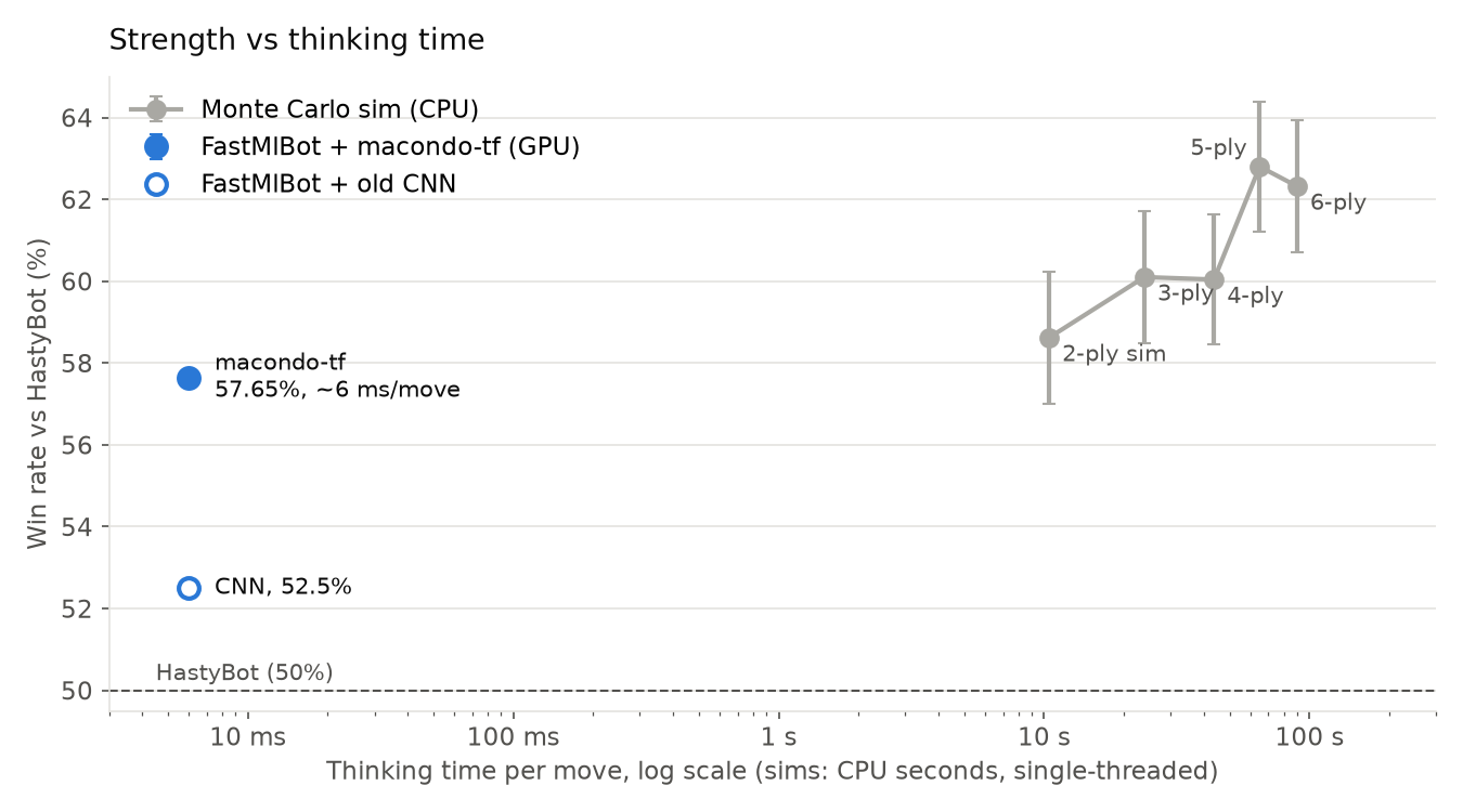
Static evaluators are supposed to be the weak, fast thing that Monte Carlo simulation improves on. So we measured how many plies of simulation it takes to beat the net. We used a simming bot of 100 candidates with fixed depths of 2 to 6 plies all game long, and no endgame or pre-endgame solver, so the comparison stays apples to apples. Each played 1,250 pairs against HastyBot:
| Bot | vs HastyBot (95% interval) | Thinking time per move |
|---|---|---|
| HastyBot | 50% | microseconds |
| FastMlBot + old CNN | 52.5% | ~6 ms (GPU) |
| FastMlBot + macondo-tf | 57.65% ± 0.18 | ~6 ms (GPU) |
| 2-ply sim | 58.62% ± 1.61 | ~10 s (CPU) |
| 3-ply sim | 60.10% ± 1.61 | ~24 s |
| 4-ply sim | 60.04% ± 1.58 | ~44 s |
| 5-ply sim | 62.80% ± 1.58 | ~65 s |
| 6-ply sim | 62.32% ± 1.62 | ~90 s |
Then we played FastMlBot against the 2-ply sim directly, 1,250 pairs:
FastMlBot paired win rate 49.04% +/- 1.56 swept 14.9% lost 16.6% spread -0.8/gameA statistical tie. A single forward pass over 50 candidates plays as well as simulating 100 candidates two plies deep, over and over. Per move, that’s more than a thousand times less work. (The sim times are single-threaded CPU seconds, and the net runs on a GPU, so this isn’t a perfectly fair race. It’s still three orders of magnitude.)
A few years ago, Joel Wapnick, a former national and world champion, replied to one of my Facebook posts about Macondo. As I remember it, his point was that bots that win by Monte Carlo simulation are in a sense “cheating”: no human sims, so what the bot does doesn’t translate to how people play. He wanted a bot that plays more the way a strong human does. I didn’t quite see his point then; to me, simulation was simply how computers think. But the comment stuck with me.
I think this net is much closer to what he was asking for. It doesn’t play out any futures. It looks at each candidate once, the way an expert glances at a position, and judges it on what it has absorbed from millions of games. And that single look plays as well as a 2-ply sim. It isn’t human, since its intuition came from 54 million bot games rather than years of tournaments, but it is intuition rather than brute force.
Simulation still wins with more depth: 3-ply is 2.5 points better, and 5-ply is 5 points better. Interestingly, the ladder goes up in steps: 3- and 4-ply are the same, and so are 5- and 6-ply.
Where does the net lose to the deep sim? We took 5-ply sim labels for about 46,000 positions and asked how often each bot’s choice matched the sim’s best play:
| Phase | Positions | Net = sim’s best | Static equity = sim’s best | Win % given up per move: net / static |
|---|---|---|---|---|
| Opening move | 15,067 | 76.2% | 65.2% | 0.09 / 0.36 |
| Early (66+ unseen) | 8,110 | 79.7% | 70.9% | 0.15 / 0.37 |
| Middle (30–65 unseen) | 14,886 | 73.8% | 66.4% | 0.24 / 0.50 |
| Late (9–29 unseen) | 8,412 | 54.4% | 43.5% | 1.32 / 2.90 |
The net beats static equity in every phase. But its weak spot is clear: in the late game it gives up over a full win-percentage point per move, ten times as much as in the opening. That’s where search, or better labels, will pay next.
Things that didn’t work
The other half of the story. Each of these got a full 100,000-pair match (except where noted), so these are real nulls, not hunches:
| Idea | Result | Compared with |
|---|---|---|
| Score the top 100 candidates instead of 50 | 57.64% | 57.65% (the net picks equity ranks 41–50 only 0.36% of the time) |
| Ownership heads (who will own each square at game end) | 57.65% | 57.65%, exactly |
| Transpose augmentation (flip half of each batch across the diagonal) | +0.30 | borderline (2.3 SE), not adopted |
| Doubling the data (27M → 54M games) | 53.13% | 53.10% |
| Rollout labels | 52.03% | 53.19% |
| Sim distillation (4 different loss functions) | 56.97–57.52% | 57.65% |
| Board-shape “energy” (Ising model) | 57.44% / 49.85% head to head | 57.65% / 50% |
| Training from scratch on self-play games | 54.45% | 55.39% (same-size HastyBot data) |
| A 6-layer distilled “student” network | 55.80%; 48.07% head to head | 57.65% (not a fit for my hardware; see below) |
A few deserve a sentence each.
Sim distillation was the most expensive dead end. We labelled every candidate of 1.26M positions with a 5-ply simulation on a 192-thread server that Gilles Blanchette of Ortograf lent us (about a week of compute), then fine-tuned the net to rank moves the way the sim does. We tried four loss functions. The best one tied the original and the worst lost 0.7 points. A full ranking of 50 candidates by a noisy sim seems to teach the net more noise than signal.
The Ising model came from a recent paper (Witteveen & Bauer, “Statistical mechanics for Scrabble”) that fits a statistical-physics model to board shapes. Its “energy” measures how unusual a board shape is. The fit worked, and energy really does predict something (high-energy boards have less extreme outcomes). But both ways we tried to use it during play did nothing: as a way to add unusual candidates for the net to score, and as a feature at the end of sim lines.
The 6-layer student. John O’Laughlin distilled macondo-tf into a smaller network for MAGPIE, the C engine he and Josh Castellano wrote (I’ve contributed to it too, though they’ve done the lion’s share). It has the same width as macondo-tf but 6 layers instead of 8: 2.8M parameters instead of 3.7M, about a quarter smaller. On my machine it didn’t pay off: it gave up about 2 points against HastyBot (55.80%) and lost to macondo-tf head to head, and it was only 6% faster, because on my setup the GPU isn’t the bottleneck. I’m still hopeful about it in some form, maybe as an even smaller student. A smaller net should matter much more where the network itself is the expensive part: on a CPU, on a laptop, or inside a search that has to evaluate thousands of positions per move.
What about an NNUE?
Last time I floated an NNUE, the tiny CPU-friendly network that made Stockfish the strongest chess engine in the world. We never built one, and I now think it probably wouldn’t work well for Scrabble. David Shin was skeptical when I brought it up, and the more I think about it, the more I agree.
An NNUE is fast for two reasons. First, its first layer is a big, sparse sum over simple features like “this piece on this square”, and a move changes only a few of them, so the network can update instead of recomputing. Second, it’s deliberately weak. Its job is to be called millions of times inside a deep alpha-beta search, and the search makes up for what the evaluation misses.
Neither fits Scrabble well. What makes a Scrabble position good or bad is mostly about combinations:
- which letters fit which hooks;
- whether a lane is usable by the tiles that are actually left;
- how your leave interacts with this particular bag.
A shallow network built on a sum of one-tile-on-one-square features is a poor fit for that kind of reasoning. Attention, where every square can look at the rack, the unseen pool and every other square, is a good fit. And Scrabble doesn’t give you the deep search that would let a weak evaluator off the hook. Hidden racks and random draws keep our searches shallow and sampled. So the evaluation itself has to be smart, not just fast.
Our own results point the same way. The spatial heads, which teach the network board geometry, were the biggest jump in this whole project. Even the 6-layer student, which is still a full transformer, gave up 2 points. I can’t prove an NNUE would fail, and I’d be happy to be wrong. But I wouldn’t bet on it.
Self-play, and what the HastyBot yardstick hides
Everything above trains on games played by HastyBot (or HastyBot with some randomness). The obvious next step, and the AlphaZero idea, is to train on the net’s own games. So we generated 3M games of macondo-tf against itself and fine-tuned on them, mixed 50/50 with HastyBot games. As a control, we did the same fine-tune with 3M fresh HastyBot games.
Against HastyBot, self-play looked like a failure:
self-play fine-tune: 57.07% +/- 0.18
HastyBot control:    57.56% +/- 0.18
Then we played them against each other:
self-play fine-tune vs HastyBot control: 50.30% +/- 0.16
self-play fine-tune vs macondo-tf:       50.37% +/- 0.16
The self-play net beats both head to head, by margins that are about 4 standard errors. Two real effects with opposite signs. A net that learns from HastyBot’s games learns how to beat HastyBot specifically. A net that learns from its own games gets better against strong opponents and slightly worse at exploiting HastyBot’s particular weaknesses.
The lesson: a match against HastyBot measures how well you exploit HastyBot, not strength in general. Any future self-play work needs a head-to-head yardstick too. It’s also why we’re shipping two models:
macondo-tf(the default): the best against HastyBot.macondo-tf-selfplay: beatsmacondo-tfhead to head.
Some positions
Here are four positions from FastMlBot’s games where the net disagreed with HastyBot’s static equity. For each one I ran a 5-ply simulation to decide who was right. Three times the sim sided with the net. One time it didn’t.
Position #1: don’t open the edge
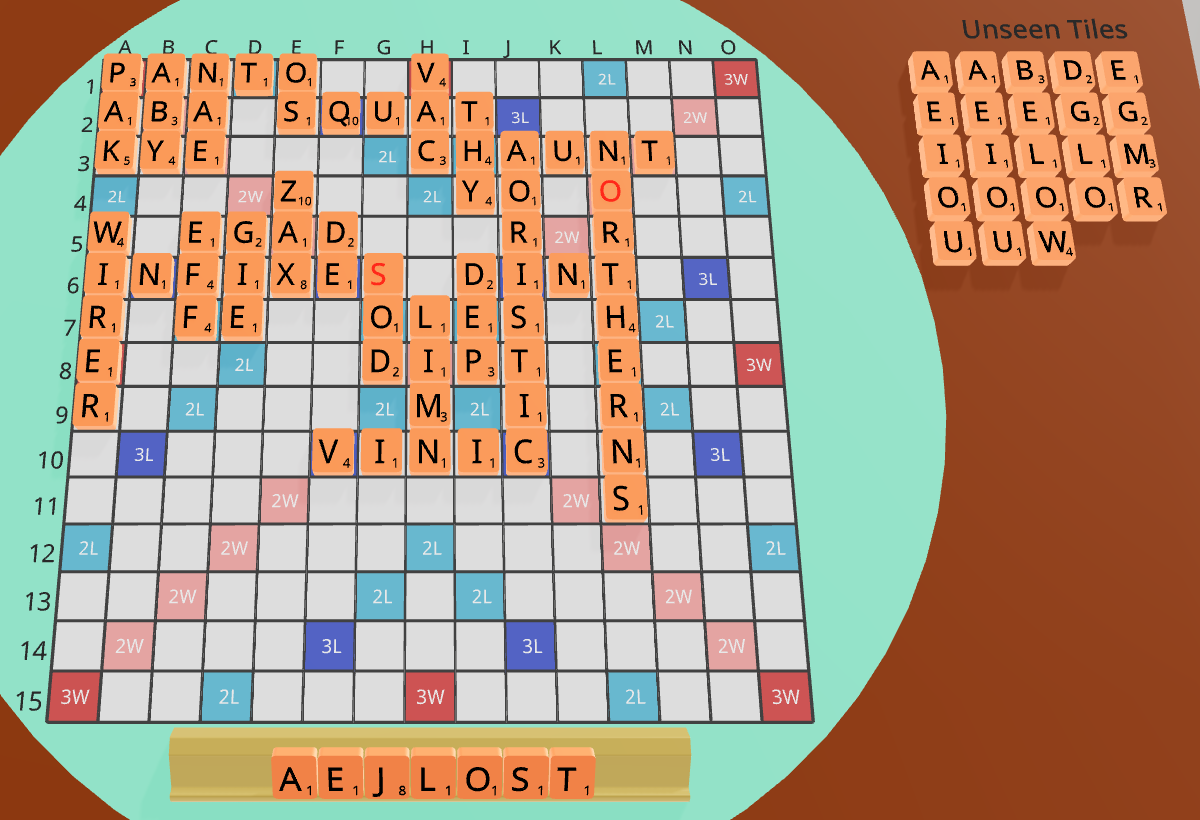
We’re down 284–303 with 16 tiles in the bag and AEJLOST. Static equity loves N1 JOSTLE for 42 points, keeping just an A. It’s equity’s #1 play by a wide margin.
The net plays 4E (Z)OA for 16, keeping EJLST. ZOA is only 13th by equity. JOSTLE puts six tiles in column N, right next to the O column, which runs between two triple-word squares. The net’s own opponent-score head expects the opponent to score 38.6 points after JOSTLE and 17.3 after ZOA.
The 5-ply sim agrees, and emphatically: ZOA wins 71.2% (± 1.2) and JOSTLE wins about 50% (± 6). That’s a 20-point swing for “don’t score 42 points”. HastyBot can’t see it, because nothing in score plus leave knows about the board.
Position #2: keep the Q
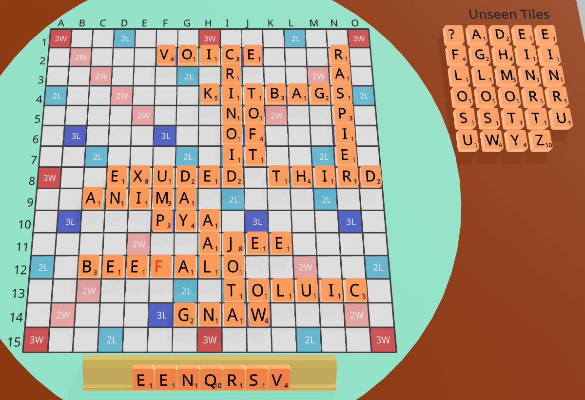
We’re up 280–276 with 22 in the bag and EENQRSV. Static equity plays H1 Q(I) for 33 on the triple-word square, unloading the Q and keeping EENRSV. Every Scrabble instinct agrees: dump the Q for 33 points.
The net plays 15J NERVES for 36, on the other triple at O15, and keeps the Q.
The sim sides with the net: NERVES 69.0% (± 3.0), QI 56.7% (± 3.4). Why? I asked Macondo’s explain command, which sims the two plays and has a language model read the sim’s statistics. Its answer is defense. The bottom row is the opponent’s best scoring lane: after QI, 28% of their replies go there, for 49 points on average, and they score 50 or more 16% of the time. NERVES takes that lane, and their 50-point replies drop to 4%.
The Q isn’t stranded, either. The QI spot at H1 stays open, and we play Q(I) there on about half of our next turns anyway. QI keeps the far better leave (EENRSV against a lone Q), but NERVES grabs the lane first and cashes the Q later. The net’s call surprised me.
Position #3: the leave, in a vowel-heavy bag
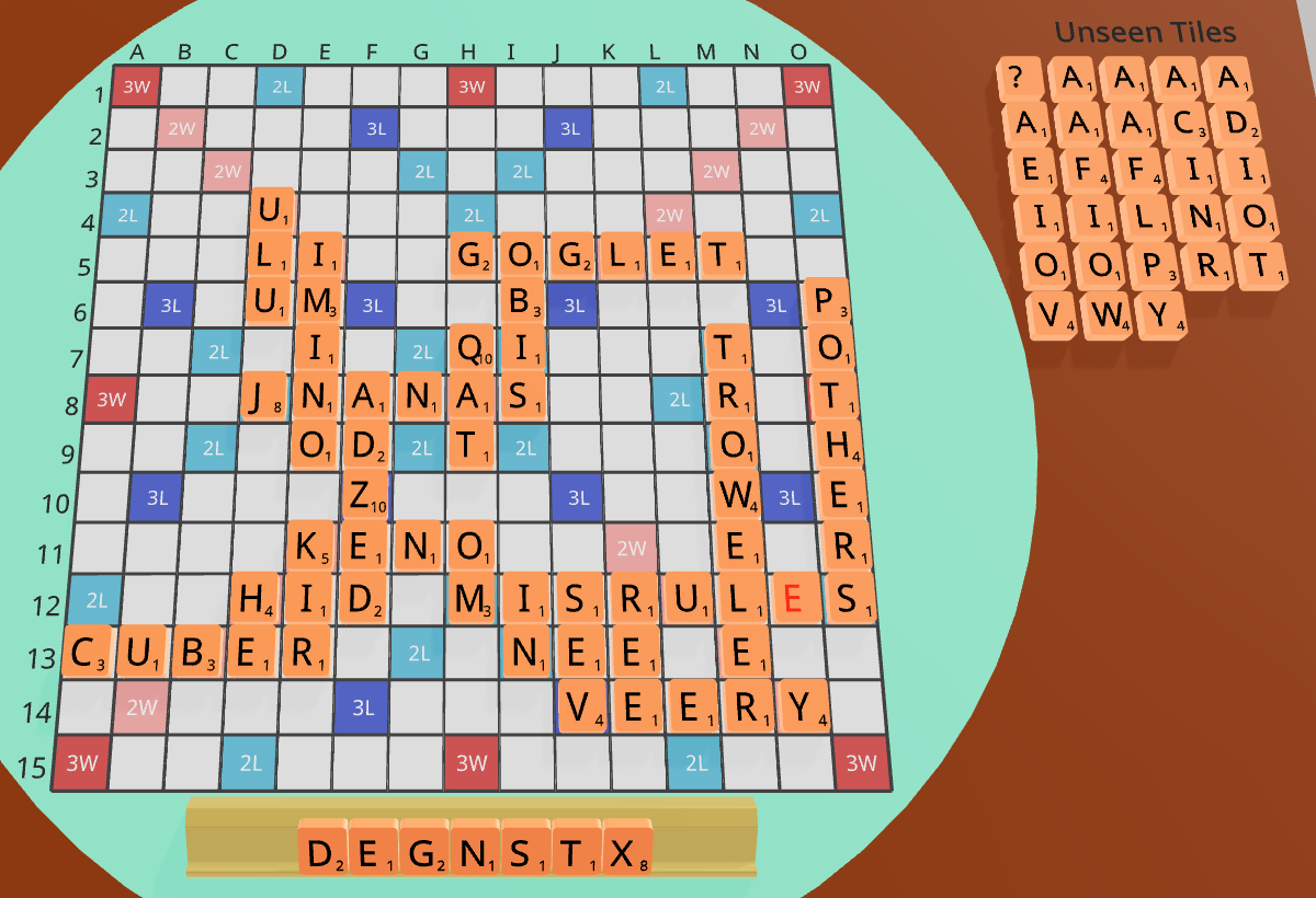
Essentially tied (286–285), 21 in the bag, DEGNSTX. Static equity plays 15F NEXTS for 43 points, keeping DG. The net plays L4 D(E)X for 22, keeping EGNST.
Look at the unseen tiles: seven A’s, four I’s, three O’s. Drawing into EGNST from that bag is a bingo waiting to happen, and the bottom row has room for one (EATINGS, TANGOES, AGNATES), the same row NEXTS would fill. Drawing into DG is not. Macondo’s explain puts our bingo chance next turn at about 46% after DEX and 8% after NEXTS. The sim: DEX 72.6% (± 2.4), NEXTS 60.9% (± 4.4). HastyBot’s leave values are averages over all bags. The net sees this bag, and this board’s hooks: its inputs include the unseen tiles and, for every empty square, which letters could legally go there. Nobody tells it whether a row has room for a whole bingo, but it likely learns that kind of thing from those inputs.
Position #4: when the net is wrong
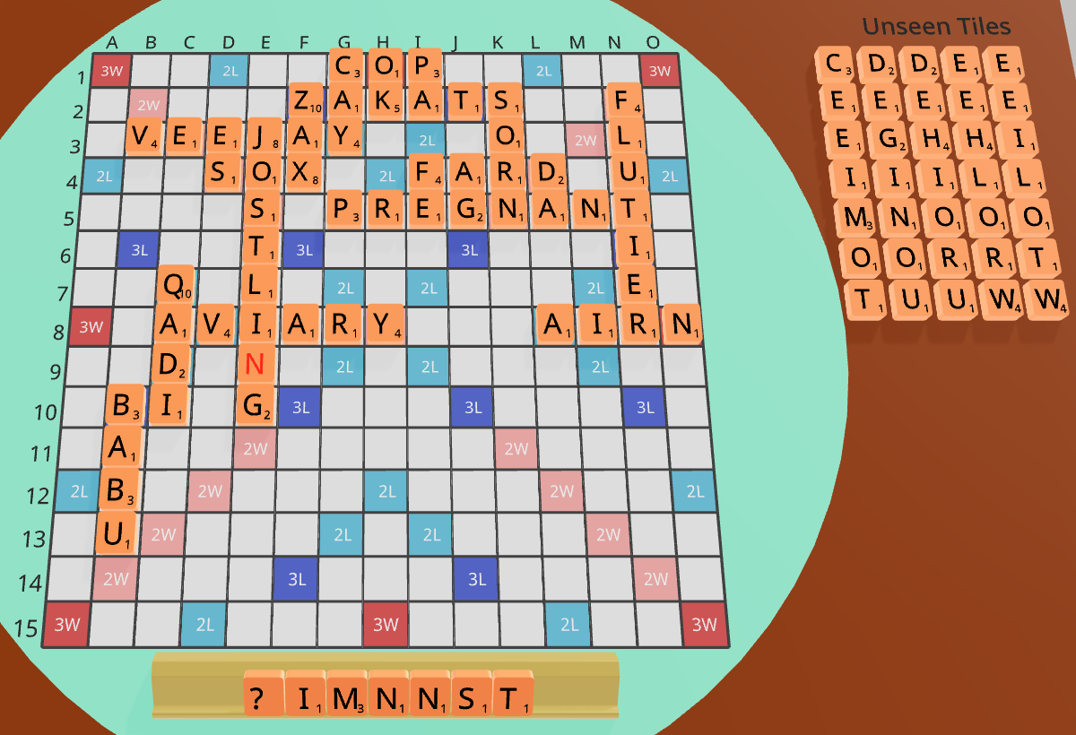
Down 254–281, 28 in the bag, ?IMNNST. There’s a 74-point bingo: L4 (DA)MN(A)TIoNS. Static equity plays it. The net plays D10 NIM, keeping ?NST, and thinks NIM wins 73.2% to DAMNATIONS’ 70.9%.
The sim says otherwise: DAMNATIONS about 74–76%, NIM 70.3%. This is the net’s most typical big mistake. When we looked at the largest disagreements between the net and static equity, most were declined bingos and big scores, and the sim sided with equity in most of them. The net sometimes falls in love with a blank leave. Its boldest deviations are its worst ones.
Engineering notes
A few things that aren’t about strength but made the work possible:
- Serving. The net runs in NVIDIA Triton as a TensorRT engine in fp16. The repo ships the portable
model.onnx, and a script compiles the engine for your card. Without a GPU, Macondo can run the samemodel.onnxon the CPU through ONNX Runtime. That’s slow, but fine for analyzing a game. - Generation speed. Self-play generation went from 113k to about 427k games per hour on one desktop. The steps: send the board planes as bytes instead of floats (they’re all 0 or 1), score only the top 16 candidates in generated games, let Triton batch requests from many games, build the feature bytes directly and patch them per candidate, and skip a word-graph optimization that slows down tiny endgame searches.
- Hardware. Most of this ran on the RTX 3070 Ti from the first post. In October I upgraded to an RTX 5070 Ti, which roughly doubled both training and match throughput. A full training run is about a day.
Who actually did the work
In the first post I said Copilot, ChatGPT and Cline wrote a vast amount of the code, with me babysitting. This time the balance shifted further. Most of this project was run by Claude Code, Anthropic’s coding agent (Claude Opus), in my terminal.
In practice it looked like this:
- I’d pick a direction (“let’s try per-square heads like David’s”).
- Claude wrote the producer and trainer changes and the tests, queued the generation, training and match jobs to run overnight, and logged every result in
experiments.md. That log is now 2,400 lines long. - When I woke up, there was a result and a recommendation for what to try next.
It also caught a surprising number of its own bugs through tests: aliased move objects in the rollout labeler, endgame labels computed from the wrong spread, a rack-dealing order that shortchanged the opponent.
It wasn’t fully autonomous. I steered the research, said no to plenty of ideas, and occasionally had to explain that “2-ply” should mean 2 plies all game long. But about 30 trained models and dozens of 100,000-pair matches in one month would have been impossible for me alone, on nights and weekends. Full disclosure: Claude also drafted this post, and I edited it.
What’s next
- The net inside BestBot. This was the obvious idea last time, and it’s even more obvious now. BestBot’s sims use HastyBot’s static evaluator to pick every move in every rollout. A rollout bot that plays like a 2-ply sim should make the sims themselves much stronger.
- The late game. The net is at its weakest with fewer than 30 tiles unseen. Better late-game labels, or handing those positions to search, is the clearest gap.
- More self-play, with a head-to-head yardstick this time.
- Other lexica. Everything here is NWL23. CSW needs its own training run.
Can I try it?
Yes. Both models are in Macondo under data/strategy/default/models/. The README’s “Using Triton” section covers building the engines, starting Triton, and choosing a model (macondo-tf is the default; set triton-model-name to macondo-tf-selfplay for the other one). Without a GPU, point Macondo at ONNX Runtime and it’ll run on the CPU.
Thanks to David Shin, whose recipe and ideas are behind most of the big jumps in this post, to Morris Greenberg for pushing the transformer idea, to John O’Laughlin for confirming the win rate and building the distilled model for MAGPIE, and to Gilles Blanchette of Ortograf for lending the 192-thread server that ran the sim labelling. If you want to help make the best Scrabble bot we can, the Woogles Discord is the place.