Bayesian Rack Inference in Macondo: Teaching a Scrabble Bot to Read Minds
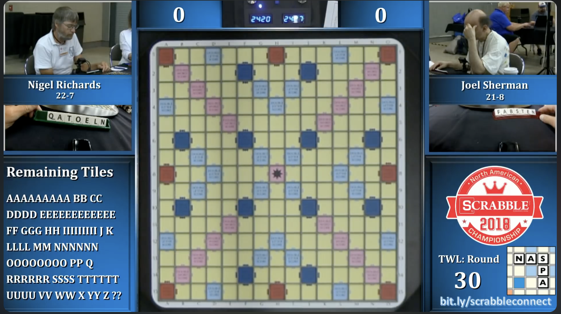
At the 2018 National Scrabble Championship in Buffalo, NY, the GOAT of all time Nigel Richards was playing against another top player and grandmaster Joel Sherman in a de-facto three-game finals for the $10K top prize. Joel needed to beat him 3 in a row to win the whole thing. In the second game (Joel won the first one), Joel opened with the rack of AENSTUU. He thought briefly before exchanging UU, his best play. Nigel had the rack AELNOQT and the commentators stated the obvious - play QAT for 24 points. There was no question in anyone’s mind about this basically automatic play.
After a minute or so, Nigel plays -OQ (exchange OQ) and one of the commentators gasps audibly. You can see the moment in this video on YouTube: https://youtu.be/xll4R_C6h-w?si=2wubjJGXBNMXUvBT&t=135
(By the way: Joel Sherman ended up winning the championship, taking all three games. Amazing feats of inference from Nigel notwithstanding.)
Key Takeaways
- QAT is the best play without inference; -OQ rises to #1 when Nigel correctly infers Joel’s strong leave
- Macondo’s new Bayesian inference engine replicates this kind of rack-reading, achieving 51.9% ± 0.8% vs BestBot (NWL23)
- Knowing your opponent’s exact leave each turn only yields 53.3% (NWL23) - barely above Bayesian inference at 51.9%
- Even knowing your opponent’s full rack each turn (full-rack oracle, CSW24) only gets you to ~62%, lower than most players expect
What Nigel Knew
Joel’s opening exchange of UU tells you a lot. He is almost certainly sitting on a very nice leave – it turns out he kept AENST, one of the best five-tile leaves in the game. He’s highly likely to bingo next turn. Playing QAT drops nice tiles for Joel to play through (A & T), handing him a minor gift, and keeps a relatively mediocre leave of ELNO. If Joel bingoes, Nigel will be at an immediate disadvantage for the rest of the game.
By exchanging OQ instead, Nigel increases his own bingo percentage - AELNT is a very good leave, and he denies Joel a couple of letters to bingo through, in case Joel misses his “fish”.
QAT is correct without inference. With inference – with Nigel reading the signal in Joel’s exchange – -OQ takes the top spot. The margin is close, but it’s there. This is exactly the problem Macondo’s new Bayesian inference feature is designed to solve.
Running infer in Macondo for this move, from Nigel’s perspective:
Inferred 1187 unique racks from 25635 iterations (4.6% acceptance), tau=0.050, ESS=510.3

Way more than chance:
 ?  S

More than chance:
 C  N  R

Slightly more than chance:
 E  I  L  T

About as expected:
 H  P

Slightly less than chance:
 A  D  G  M  Z

Less than chance:
 B  F  K  O  V  X

Way less than chance:
 J  U  W  Y

Unpossible:
 Q
Running infer details shows:
Top inferred racks (by Bayesian weight):
  Rank  Leave       Weight      Wt %
  1     AGILN       0.9504      0.7
  2     ADERT       0.7625      0.6
  3     DEISS       0.7594      0.6
  4     AINOT       0.7533      0.5
  5     DEIRT       0.7327      0.5
...
along with some more per-tile details.
Then, you can sim with these inferences:
sim -plies 5 -stop 99 -useinferences weightedrandomracks
Play                Leave         Score    Win%            Equity
(exch OQ)           AELNT         0        43.28±0.73      -37.59±1.77
 8G QAT             ELNO          24       43.11±0.73      -37.17±1.71
It’s close, but if you run this 100 times, the exchange wins about 73% of the time.
(For more about how Macondo’s simulation engine works, read a technical deep-dive on truncated Monte Carlo simulation in Scrabble: https://domino14.github.io/macondo/howitworks.html#monte-carlo)
Replicating It in Macondo
Macondo v0.13.0 (merged April 25, 2026) introduces SIMMING_INFER_BOT, a bot that performs Bayesian rack inference before each simulation pass. You can download the latest Macondo version here: https://github.com/domino14/macondo/releases
To run it in autoplay mode:
autoplay -botcode1 SIMMING_INFER_BOT -botcode2 SIMMING_BOT \
  -numgames 1000 -logfile results.txt
autoanalyze results.txt
(Note: this is slow and can take several days if you don’t have a supercomputer!)
Before each move, the inference engine runs for up to 20 seconds, examining what the opponent played and asking: given that they made that play, what leave are they most likely holding? That information then biases the simulation.
The relevant parameters:
| Parameter | Default | Purpose |
|---|---|---|
tau |
0.05 | Softmax temperature on log-odds scale |
inferenceTimeSecs |
20 | Time budget per turn |
inferenceSimIters |
200 | Mini-sim iterations per candidate leave |
maxEnumeratedLeaves |
750 | Exhaustive mode threshold |
The Old Approach: Static Inference
Before the current method, Macondo had a simpler, faster inference system. Instead of running mini-simulations, it would look at the engine’s top moves ranked by static equity (immediate score plus leave value) and check whether the opponent’s actual play appeared somewhere in that list within a certain equity threshold. If it did, that rack was considered plausible. If it didn’t, the rack was discarded.
This sounds reasonable. It’s fast and it requires no simulation at all, and it’s often accurate.
The problem is that static equity is a single-turn evaluation. It doesn’t model what the opponent is planning.
Consider a setup play - a play that sets up a Q on your rack for a huge score next turn. The equity-ranked list would often put such a play somewhere near the bottom, well below the threshold. Static inference would conclude: “this rack doesn’t explain the play” and throw it out.
The result is systematic bias. Static inference works fine when opponents play straightforwardly, but it fails exactly when the opponent is being clever. It can only “find” a setup by accident, if the setup happens to also score well. It can’t represent the plays that require looking ahead.
Win probability from simulation doesn’t have this problem. A mini-sim runs out the game a couple of turns from a given rack and position. Setups show up as high-win% plays because the simulation sees the bingo or high scoring play on turn 2. Exchanges show up as high-win% plays when the leave is great, taking into account the board position. The move the opponent actually made gets evaluated on the same scale as every alternative, and that scale is the right one.
That’s what the current method uses, and why it produces better inference despite being slower.
The Bayesian Math
The core update is the standard Bayesian posterior:
P(leave | play) ∝ P(play | leave) × P(leave)Breaking this down:
- P(leave | play) – what we want: given that the opponent just made that specific play, how likely is it they’re holding this leave?
- P(play | leave) – the likelihood: if the opponent were holding this leave, how probable would it be that they’d make exactly that play?
- P(leave) – the prior: before seeing the play, how likely was this leave just from the bag draw?
We compute this for every plausible opponent leave, normalize, and use the resulting weighted distribution to guide simulation.
Why Softmax on Log-Odds Instead of Raw Win Probabilities
To estimate P(play | leave), we run a mini-simulation: given a hypothetical opponent rack (tiles played + candidate leave), what are the win probabilities of all their legal moves? Then we ask: how likely were they to have chosen the move they actually made?
The naive approach – softmax over raw win probabilities – is mathematically wrong. Win probabilities are already sigmoid-compressed, bounded in (0, 1). Applying softmax to them distorts sensitivity at the extremes. The right approach is to convert to log-odds (logit) first, then apply softmax with a temperature parameter τ.
func logit(p float64) float64 {
    if p < logitEps {
        p = logitEps
    } else if p > 1-logitEps {
        p = 1 - logitEps
    }
    return math.Log(p / (1 - p))
}

func softmaxLikelihood(plays []*montecarlo.SimmedPlay, targetMove *move.Move,
                       b *board.GameBoard, tau float64) (float64, float64) {
    targetWinProb := math.NaN()
    maxLogOdds := math.Inf(-1)
    for _, sp := range plays {
        lo := logit(sp.WinProb())
        if lo > maxLogOdds {
            maxLogOdds = lo
        }
        if movesAreTheSame(sp.Move(), targetMove, b) {
            targetWinProb = sp.WinProb()
        }
    }
    if math.IsNaN(targetWinProb) {
        return 0, 0
    }
    sum := 0.0
    for _, sp := range plays {
        sum += math.Exp((logit(sp.WinProb()) - maxLogOdds) / tau)
    }
    return math.Exp((logit(targetWinProb)-maxLogOdds)/tau) / sum, targetWinProb
}
The maxLogOdds subtraction before math.Exp is a standard numerical stability trick – it prevents overflow without changing the result. τ = 0.05 is the default, tuned to assume near-optimal play. Lower τ sharpens the distribution (punishes suboptimal choices more), higher τ spreads weight more permissively.
Why log-odds? The sigmoid compression problem shows up most clearly at the extremes. Consider two pairs of moves: one with win probs of 0.51 and 0.53, another with win probs of 0.95 and 0.97. Both pairs are separated by the same raw probability gap of 0.02, so raw softmax treats them identically. But they represent very different quality gaps. The first pair is 1.04:1 odds vs. 1.13:1 odds - a genuinely close call. The second pair is 19:1 odds vs. 32:1 odds - a huge quality difference that the sigmoid has compressed into a tiny slice near 1. Log-odds undoes that compression: logit(0.53) - logit(0.51) ≈ 0.08, while logit(0.97) - logit(0.95) ≈ 0.54. The same raw gap becomes 7x larger on the log-odds scale when it occurs near an extreme, which is exactly the right behavior. Equal differences in log-odds correspond to equal multiplicative differences in odds - and that’s the right scale for comparing move quality.
The Hypergeometric Prior
P(leave) – the prior – is the probability of drawing that specific leave from the bag. This is a multivariate hypergeometric distribution.
If the bag has N tiles total, and the opponent is drawing k tiles, the log-probability of drawing a specific leave is:
log P(leave) = Σ_t log C(bagMap[t], leaveCount[t]) − log C(N, k)where the sum is over tile types t. We compute binomial coefficients via math.Lgamma for numerical stability:
func combinatorialPrior(leave []tilemapping.MachineLetter, bagMap []uint8) float64 {
    leaveCounts := map[tilemapping.MachineLetter]int{}
    for _, t := range leave {
        leaveCounts[t]++
    }
    N := 0
    for i, c := range bagMap {
        N += int(c)
        if leaveCounts[tilemapping.MachineLetter(i)] > int(c) {
            return 0 // impossible – tile not in bag
        }
    }
    k := len(leave)
    logP := -logBinomial(N, k)
    for t, lc := range leaveCounts {
        logP += logBinomial(int(bagMap[t]), lc)
    }
    return math.Exp(logP)
}

func logBinomial(n, k int) float64 {
    if k < 0 || k > n {
        return math.Inf(-1)
    }
    lgn, _ := math.Lgamma(float64(n + 1))
    lgk, _ := math.Lgamma(float64(k + 1))
    lgnk, _ := math.Lgamma(float64(n - k + 1))
    return lgn - lgk - lgnk
}
This gives us the exact probability of any leave given the current bag.
Exhaustive Enumeration vs. Monte Carlo Sampling
When the leave space is small (750 or fewer distinct leaves), we enumerate every possible leave exactly. We sort by prior probability descending and use a 1% early-exit on the low-probability tail to stay within the time budget. Each leave gets its own mini-sim, run in parallel across threads. The weight for each leave is:
weight = P(leave) × P(play | leave)When the leave space is large, we switch to Monte Carlo sampling. SetRandomRack draws leaves from the hypergeometric prior implicitly – it’s literally sampling from P(leave). So the weight becomes:
weight = P(play | leave) [likelihood only – prior already baked into the sampler]This is importance sampling: the proposal distribution IS the prior, so you don’t double-count it. After enough samples, the weighted collection approximates the full Bayesian posterior.
The Sigmoid Confidence Gate
After inference, we have a weighted list of probable opponent leaves. But how aggressively should the simulation use them? If we only found 3 plausible leaves, we shouldn’t be overconfident. If we found 50, we can commit harder.
A sigmoid function governs this:
α = 0.95 / (1 + exp(−(N − 10) / 5))where N is the number of distinct inferred racks. In each simulation iteration, with probability α we sample from the inferred distribution; with probability (1 - α) we draw a fully random rack.
| N (inferred racks) | α (use inference) |
|---|---|
| 3 | ~0.19 |
| 10 | ~0.48 |
| 20 | ~0.79 |
| 50 | ~0.93 |
When we do sample from the inferred distribution, we use weighted cumulative selection – proportional to posterior weight.
What the Results Actually Show
Here’s what we found after running 10,000+ simulated games per condition (necessary to get ±1% confidence at 95% CI – this takes real compute time):
| Scenario | Win Rate vs BestBot |
|---|---|
| Inference bot (τ = 0.05, NWL23) | 51.9% ± 0.77% |
| Oracle bot (knows opponent’s leave, NWL23) | 53.3% ± 1% |
| Oracle bot (knows opponent’s leave, CSW24) | 52.8% ± 1% |
| Going first advantage | 56–57% |
| Full-rack oracle (knows opponent’s full rack, CSW24) | ~62% |
The Oracle bot is a hypothetical: it knows its opponent’s exact rack leave every single turn. No inference needed – perfect information. And it only wins 53.3% of the time in NWL23, 52.8% in CSW24. (The two are within the margin of error of each other.)
Our Bayesian inference bot, working from noisy signals, achieves 51.9%. That’s… close to the same! And both are well below the first-move advantage.
We ran a (brief) second oracle experiment: what if the bot knew not just the opponent’s leave after every move, but their full rack (all seven tiles) every single turn? That’s a dramatically stronger information advantage. In CSW24, it wins ~62% of the time. Also a bit lower than expected.
When I posted this to a Facebook Scrabble forum – asking whether players would rather go first, or know their opponent’s exact leave after every play – the consensus seemed to be the latter. “Obviously know the racks, that’s so much more information.” It’s not even that close.
When I first shared the result in our Discord server, people were convinced I’d made a mistake somewhere in the methodology. It wasn’t until someone else (John O’Laughlin of Quackle fame) independently replicated the experiment that the incredulity faded. World #2 David Eldar summed up the sentiment perfectly:
“deep down we all want this to be a poker-like soulread game”
He’s right - we want it to be true! Scrabble feels like it should reward reads the way poker rewards reads. But the bag randomizes so aggressively, turn after turn, that even perfect information decays fast. By turn 3, whatever you inferred on turn 1 is often mostly gone.
This doesn’t mean inference is useless – 52% vs 50% is a real edge, and in tournament play small edges compound. But it’s humbling… the bag is a brutal equalizer.
The Strange Sensitivity of τ
When you have a continuous parameter like τ, the natural expectation is a smooth response curve: performance rises as τ approaches the optimum, peaks, then falls off the other side. Tune τ too low and the model is overconfident; too high and it becomes too permissive. You’d draw a hill. That’s not what we found.
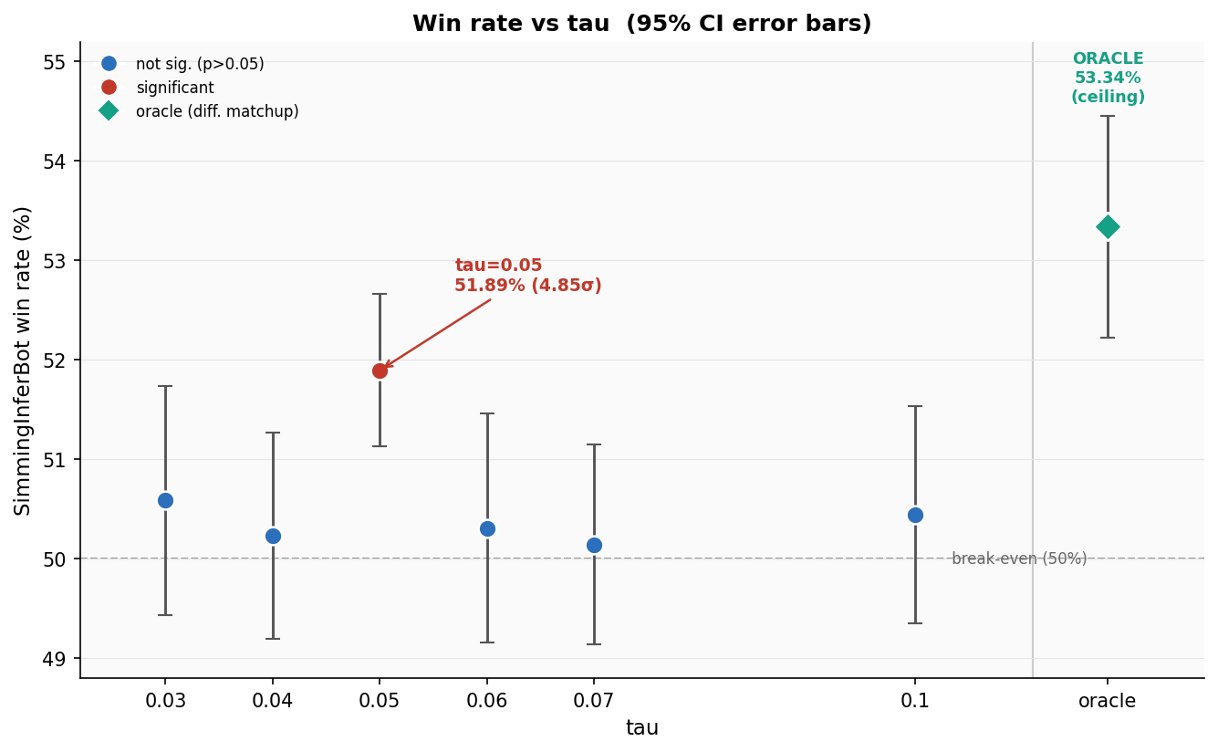
At τ = 0.05, the inference bot wins 51.89% of games, a 4.85σ effect. That’s just below the 5σ bar physicists use for “discovery,” which corresponds to roughly one-in-a-million odds that the result is a random fluctuation. It’s real!
Every other τ value tested (0.03, 0.04, 0.06, 0.07, 0.1) has a 95% confidence interval that straddles 50%. They are statistically indistinguishable from noise. The immediate neighbors on either side, 0.04 and 0.06, are dead. This isn’t a hill with τ = 0.05 at the top. It’s a spike.
The obvious objection is multiple comparisons: if you test six τ values and only look for any one of them to be significant, you inflate your false-positive rate. Fair. But a Bonferroni correction for six tests shifts the significance threshold from ~2σ to ~2.6σ. A 4.85σ spike doesn’t just survive that correction; it dominates it. The effect is real, not an artifact of data dredging.
What’s actually going on here? The more we think about it, the more we suspect the primary culprit is mini-sim noise, not opponent rationality.
Each candidate leave gets evaluated with 200 mini-sim iterations. At 200 samples, the standard error on a win probability near 50% is roughly ±3.5 percentage points. On the log-odds scale, that translates to about ±0.14 log-odds units of noise per move. Now look at what a low τ does to that noise: the softmax weight is proportional to exp(logit/τ). At τ = 0.03, a 0.14 log-odds noise swing between two moves produces a weight ratio of exp(0.14/0.03) ≈ 100x. At τ = 0.05, the same noise gives exp(0.14/0.05) ≈ 16x. At τ = 0.10, it’s exp(1.4) ≈ 4x. Below τ = 0.05, the softmax is essentially making hard commitments based on what is largely ranking noise in the mini-sim estimates. It confidently declares the observed move “wrong” for a given rack just because a noisy estimate flipped the ranking, and discards that rack even though it’s perfectly consistent with the observed play. The posterior collapses not because the opponent plays suboptimally, but because the likelihood estimates aren’t clean enough to support that level of sharpness.
There’s also a secondary rationality effect: BestBot isn’t a perfectly deterministic optimizer, so a very low τ additionally punishes racks whose best move differs even slightly from what was played. But this is a second-order issue. The noise story is more direct, and it has a clean experimental test: if you increase inferenceSimIters from 200 to 2000, the noise drops by a factor of sqrt(10) and the optimal τ should shift noticeably lower. If it does, noise is dominant. If it doesn’t move, rationality mismatch is the real driver. This is exactly why the 2D grid search over τ and inferenceSimIters that Morris suggested makes mechanistic sense: the two parameters aren’t independent. They interact through noise, and the optimal τ for 200-iteration mini-sims may be quite different from the optimal τ for 1000-iteration mini-sims.
What’s Next
We’re still searching for the optimal τ. It likely varies by opponent – a player who always takes the BestBot-approved play is easier to infer against than one who plays more creatively. τ can also potentially adapt over the course of a game as you accumulate evidence about your opponent’s style.
Morris Greenberg suggested several promising directions for a more systematic τ search. The approach we’ve used so far is a coarse manual sweep; Morris proposed a proper grid search with finer resolution, evaluating each candidate τ on a held-out set of games to avoid overfitting to the BestBot matchup specifically. He also suggested a 2D search over τ and the mini-sim iteration count together, since the two parameters interact: a lower τ (sharper posterior) only works well if the mini-sims are precise enough to rank moves reliably, and cheap mini-sims may need a more forgiving τ to compensate for their noise. These ideas will shape the next round of experiments.
Increasing the number of iterations per mini-sim can only help, too, as well as increasing their plies and number of considered plays. However, this can also result in a prohibitively slow bot!
One idea we haven’t implemented yet is sequential inference - carrying the posterior forward across turns. Right now, each turn’s inference starts fresh: we compute P(leave | play) from scratch using the flat hypergeometric prior, as if we’d never seen the opponent before. But that throws away information. If you inferred on turn 3 that your opponent is very likely holding an S and a blank, and they only played two tiles on turn 4, some of those tiles are probably still on their rack. The turn-3 posterior should be informing the turn-4 prior.
Concretely: after the opponent plays K tiles on turn N, their rack for turn N+1 consists of their turn-N leave (which you just inferred) plus K newly drawn tiles from the bag. So the prior for turn N+1 isn’t the flat bag distribution - it’s the convolution of your turn-N posterior over leaves with the hypergeometric draw distribution for those K new tiles. In principle this is straightforward Bayesian updating; in practice the posterior is a distribution over thousands of possible leaves and computing the convolution efficiently is non-trivial. But it’s the right thing to do, and the information gain should compound over time, especially in games where the opponent plays conservatively and carries similar tiles across multiple turns.
In the coming weeks, BestBot on Woogles will be updated to run inference. This should make it a more formidable opponent – and, perhaps more importantly, a more human-like one. A bot that actually thinks about what you’re holding is a bot that plays the way the best humans play. (It might also be more fun to play against!)
If you want to experiment yourself, clone Macondo and try autoplay with SIMMING_INFER_BOT. Play with τ, inference time, and enumeration thresholds and let me know what you find.
(For more about BestBot - the best Scrabble AI out there, powered by Macondo - read this blog post: https://blog.woogles.io/posts/2025-05-04-the-mathematics-and-algorithms-behind-bestbot/)
Important note regarding Monte Carlo
Truncated Monte Carlo sampling is still the best method we have throughout most of the game for playing a good game of Scrabble. BestBot uses this and the number of people who can beat it in a 100-game series can probably be counted on one hand.
But, we all know it has its disadvantages - mostly around the fact that it uses a pure static analyzer to do the rollout. I talk about this in my article on using CNNs to do static evaluation. A neural network-based static evaluator can potentially do much better than the static evaluator we have now. It’s very possible therefore that the 53% or so number that represents the edge the Oracle bot has over BestBot could be higher if we were using a better static evaluator. So this doesn’t necessarily represent a hard limit for the advantage that we can get from inference. But my bet is that it would still be pretty close and not as overwhelming as one would think.
Examples
Here are a few interesting positions where simmed inference gives some good results. Nigel is far from the other player who can do setups, although his are often known to be legendary. For more on these plays you can watch Will Anderson’s videos Volume 1 and Volume 2.
Position 1
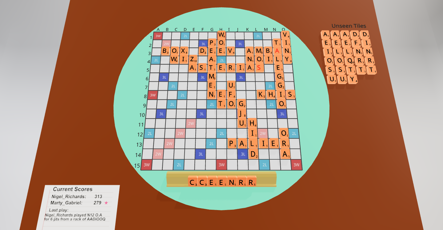
In the above position, Nigel has just played the stunning N12 O(R)A holding ADIOQ. This was round 4 of the 2010 Causeway Challenge vs. Marty Gabriel, played with the CSW07 lexicon. He is setting up 15L QADI for 77 pts!
The results show:
Way more than chance:
 D  I  Q

More than chance:
 A  L  N
With every other letter being way less than chance or impossible. The sim engine thinks Marty should block with O14 RE at all costs, even though that would normally be a pretty bad move. It’s that desperate.
Position 2
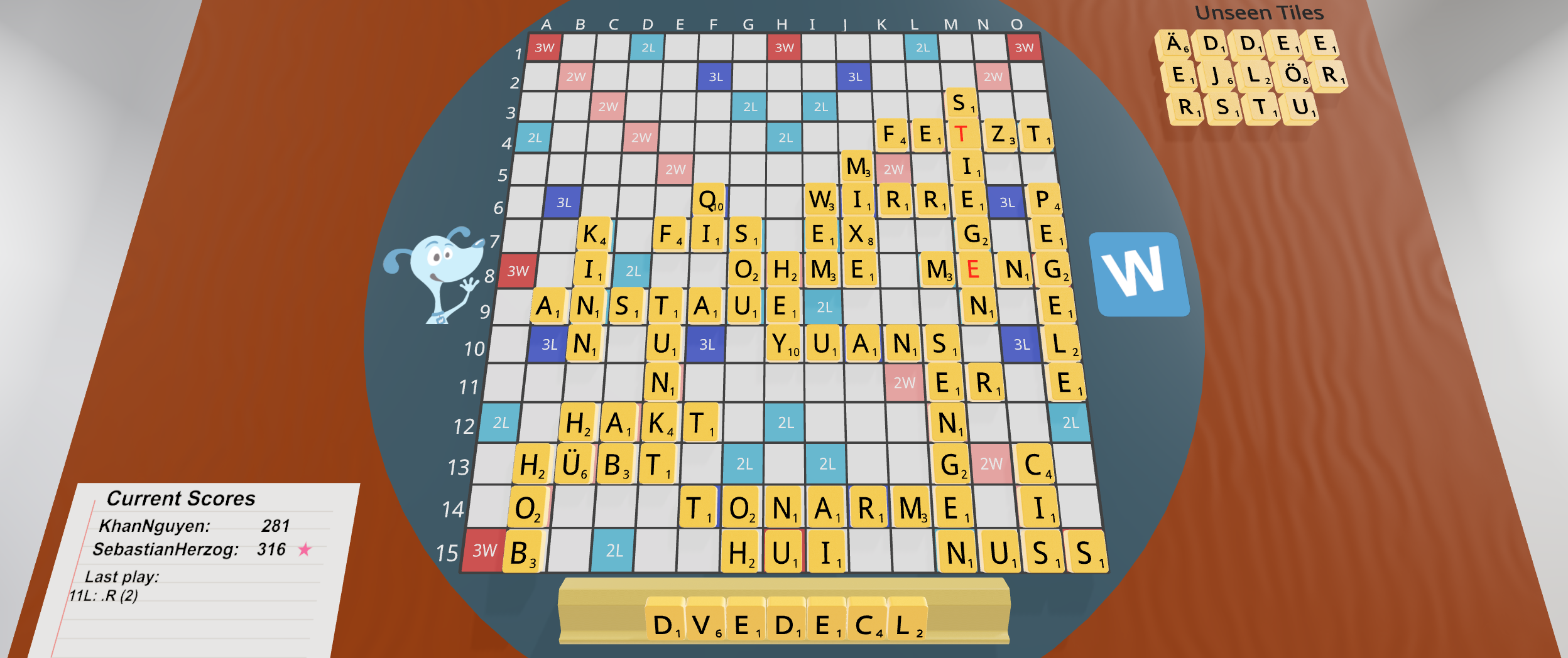
Inference works in other languages too. The above position happened between Khan Nguyen and Sebastian Herzog. Khan is the 2025 National Scrabble Champion in German. His last move is 11L (E)R for just two points.
Khan is setting up a big parallel play making ÖL to try to steal this game; the Ö is worth 8 points so this can easily be a 50+ point play.
The inference shows this:
Way more than chance:
 Ö

More than chance:
 L

Slightly more than chance:
 D  R

About as expected:
 T

Slightly less than chance:
 J  S  U

Less than chance:
 Ä  E
Indeed, Khan kept DEÖRTU, trying to set up ÖL/ERDE. (Note that ERLE is also a word in German).
With this inference Macondo suggests that Sebastian should play K9 A(N)D to block the huge hotspot.
Position 3
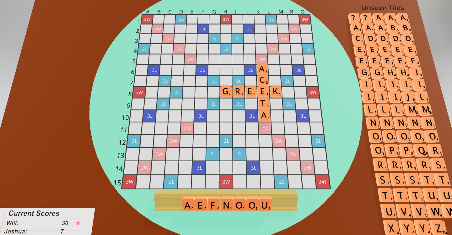
This game took place during Round 8 of the 2019 National Scrabble Championship in Reno, NV. Josh Sokol played AC(E)TA in the above position vs Will Anderson, setting up a huge Z spot in two different places. Beautiful! He kept ZIT on his rack.
Way more than chance:
 A  Q  Z

More than chance:
 C  D  T

Slightly more than chance:


About as expected:
 E  W
Imagine that we did not sim using inferences. In this case, the simulator thinks that Will should play J10 FOU keeping AENO for 27 points.
Play                Leave         Score    Win%            Equity
J10 FOU             AENO          27       59.21±0.76      -23.59±1.77
J10 FOO             AENU          27       58.35±0.78      -25.64±1.78
 J4 OOF             AENU          27       57.99±0.78      -26.37±1.79
 J4 OAF             ENOU          27       56.84±0.82      -29.07±1.87     ❌
However, simming with inferences on immediately makes I6 UN(R)OOF jump to the top!
Play                Leave         Score    Win%            Equity
 I6 UN(R)OOF        AE            11       54.81±0.92      -34.12±2.03
J10 FOO             AENU          27       52.06±1.03      -39.76±2.33     ❌
J10 FOU             AENO          27       52.05±1.04      -39.87±2.30     ❌
 J4 OOF             AENU          27       50.81±1.51      -42.76±3.36     ❌
UN(R)OOF scores very little and keeps a mediocre leave, but it blocks both Z spots. It should definitely be played here.
Frequently Asked Questions
What is rack inference in Scrabble?
Rack inference is the process of deducing what tiles your opponent is holding based on the moves they’ve made. Strong human players do this intuitively; Macondo’s Bayesian inference engine formalizes it mathematically using Bayesian posterior updates over the space of possible opponent leaves.
How does tau (τ) affect inference quality?
τ is the temperature of the softmax applied to log-odds win probabilities. Lower τ sharpens the distribution, assigning most weight to the move the opponent “should” have made. τ = 0.05 works well for near-optimal play; higher values are more forgiving of suboptimal choices. We’re still investigating the optimal value.
What is a mini-sim?
A mini-sim is a fast Monte Carlo simulation. Macondo does hundreds of these, multi-threaded, during the inference step. The goal is to do around 200 2-ply iterations with many different rack leaves to see how far the opponent’s best play is separated from the top play, and thus, when combined with the tau value, how likely a rational opponent is to have made that play given that they held that rack.
Why does knowing your opponent’s exact leave only help 53.3%? And why does knowing their full rack each turn only get to ~62%?
Because Scrabble’s bag randomizes so aggressively each turn. Even with perfect leave information, you can only act on it for one turn before both players draw new tiles. The full-rack oracle is more powerful (62%) - it sees all seven of your opponent’s tiles each turn, not just what they kept - but it’s still constrained by the same fundamental entropy: knowing your opponent’s rack doesn’t always mean you can do too much against it.
How many games are needed to measure a 1% win-rate difference?
At least 10,000 simulated games to achieve ±1% confidence at the 95% confidence level. Each game takes time even at bot speeds, which is why these experiments are compute-intensive. Much thanks to Gilles of Ortograf for letting me use his 192-core behemoth of a computer to run all of these experiments in a reasonable time frame.
Where can I try the inference bot?
Clone Macondo on GitHub and use the autoplay command with -botcode1 SIMMING_INFER_BOT. (You can also try SIMMING_INFER_BOT_NO_EG, which avoids playing an endgame/pre-endgame, for speed purposes) BestBot on Woogles.io will also be updated to use inference soon; stay tuned.
Conclusion
The soulread fantasy doesn’t quite survive contact with the bag. Rack inference helps - ~52% is a real edge - but knowing your opponent’s leave every single turn only gets you to 53.3%. Going first beats perfect leave information! That took a while to believe.
It’s not that inference is useless. It’s that Scrabble is more random than it feels when you’re playing it. The bag keeps reshuffling your read away. We’ll keep tuning τ, running more experiments, and see if the numbers move. But I’m not expecting a revelation - variance always wins.
Acknowledgements
Thanks to Morris Greenberg (PhD candidate, Department of Statistical Sciences, University of Toronto) for suggesting the Bayesian framework that became the foundation of this implementation, and for several ideas around systematic τ optimization that will shape future work. Morris’s research focuses on Bayesian methods applied to high-dimensional data, and his framing of the leave-inference problem as a proper Bayesian posterior update was the key conceptual move that made this approach rigorous.
Thanks also to Gilles of Ortograf for access to his 192-core machine, which made running 10,000+ games per condition practical, and to John O’Laughlin for independently replicating the oracle experiment results.